Asset Monitoring and Predictive Maintenance
Sponsored by FPoliSolutions, LLC
Table of Contents
Project details
Large engineered systems such as nuclear power plants consist of thousands of interconnected components.
Components eventually wear out over time which may lead to strange anomalies, faults, and system failures.
Failures may force shutdowns and are expensive to repair. Worst-case scenarios endanger public health and safety.
It is therefore critical to monitor components and understand when they must be repaired BEFORE a failure occurs.
Components are monitored in many ways. One common approach is to record vibrations.
Vibrations give insights into the dynamic response of the component.
Vibrations can tell you if the component characteristics change over time.
Certain changes may mean the component is wearing out and should be repaired before it fails.
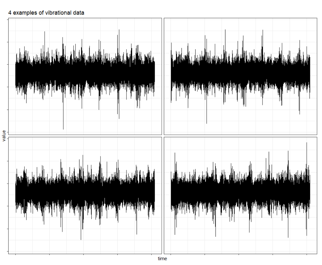
However, vibrational data are challenging to work with. Examples of vibrational data are shown below.
They are high-frequency time series signals. Patterns are hidden in the signals.
FPoliSolutions finds the patterns within the signals and monitors how those patterns evolve over time.
Certain pattern changes are associated with the component wearing out.
Finding those changes early prevents failure!
Finding those changes requires training MODELS. The models are used to PREDICT if the component has worn out and needs to be replaced.
However, failures do NOT occur all that often. This leads to significant challenges in properly training the models!
The models need to observe failures, but we do NOT want the systems to fail.
You will learn why RARE events are so challenging to model later!
It is therefore difficult to properly collect and assemble training data for predictive maintenance applications.
Computer experiments to study patterns
Computer simulations can help overcome certain challenges because the simulations are based on physical theory and engineering best practices.
Simulations are used to generate supplemental data of possible failure states.
The simulated data can be added to the existing set of real data to help train more accurate models!
The simulated data consist of higher failure rates compared to real data, because the simulations are specifically designed to induce failures.
The simulations generate vibrational data consistent with real vibrational measurements. Thus, the simulations generate high-frequency time series signals! Patterns can be extracted from those high-frequency signals.
How those patterns are extracted from the signals were not discussed here. The patterns are provided to us.
We will work with the simulated patterns. You will train models to CLASSIFY a simulated failure given the simulated patterns.
Data
- The data are provided in the CSV file training_data.csv.
- The columns correspond to different patterns extracted from the data.
- The column naming convention indicates the feature extraction approach used to generate the variables.
- X – Approach 1 at extracting patterns from the signals
- Z – Approach 2 at extracting patterns from the signals
- V – Approach 3 at extracting patterns from the signals
- The column letter is followed by a number. Each feature extraction approach includes numerous patterns.
- Approach 1 has 25 columns: X01 through X25
- Approach 2 has 9 columns: Z01 through Z09
- Approach 3 has 29 columns: V01 through V29
- The output is named Y and is a binary variable.
- The output is encoded as:
- Y = 1 is a FAILURE
- Y = 0 is NOT a failure
- The models must predict the PROBABILITY of FAILURE given the INPUT patterns (the X, Z, and V columns).
Project instructions
- This project has 2 primary goals:
- Train a model that accurately classifies failure (Y=1).
- Identify the most important inputs that influence the failure probability.
- We will need to appropriately explore the inputs BEFORE training models.
- Make sure you study the RELATIONSHIPS between the inputs!
- We must use an appropriate validation scheme to select the best model!
Steps
We have divided our project into 6 parts: EDA and Preprocessing, Cluster Analysis, Models, Performance, Prediction, and Bonus. We summed up the summaries in Mains. You will get these files with codes in jupyter notebook and HTML folders in Github. Introduction has been given so far. Let us start with the EDA.
| EDA and Preprocessing | Cluster Analysis | Models | Performance | Prediction | Bonus |
|---|---|---|---|---|---|
| Plotting necessary data, Standardization, Removing skewness, PCA | KMeans, Hierarchical clustering | 7 logistic regression models and accuracy on training data | testing on manually created data | Gridsearch, lasso, ridge, elastic net | SVC, Neural net |
| Python | Python | Python | Python | Python | Python |
EDA and Preprocessing
We can see that the input features are bell-shaped but some of them are left or right-skewed e.g., Z07, Z09, and V02 are left-skewed and V28, V29, and Z08 are right-skewed. We can also see minor bi-modality with X19.
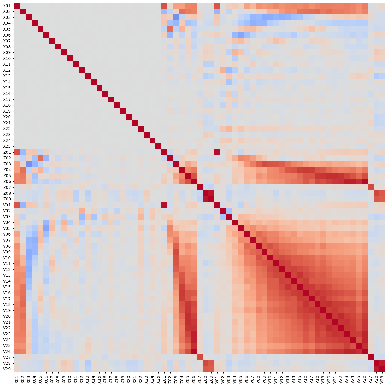
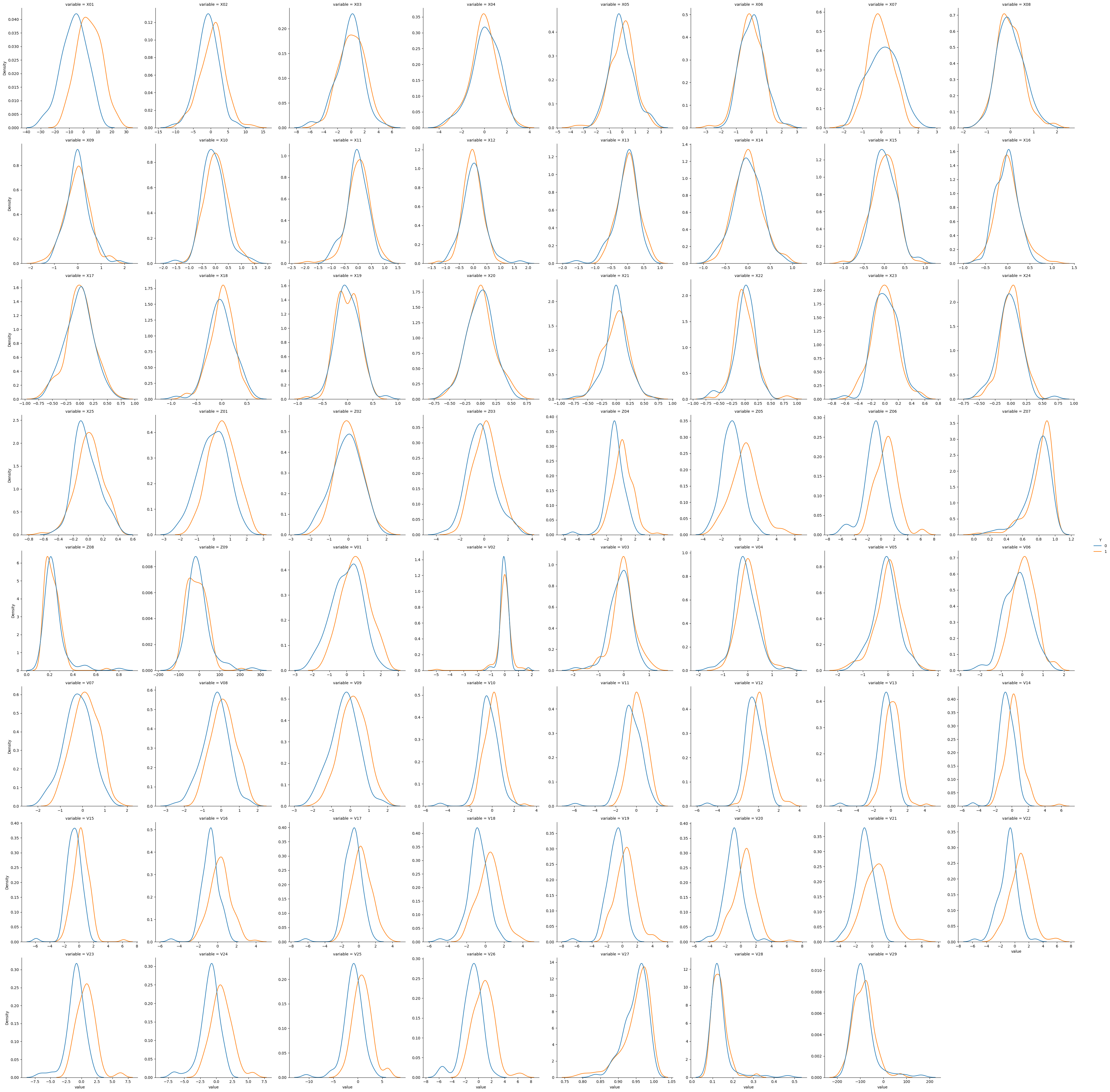 Hence we needed to use log transformation to remove skewness as we will use KMeans later on. We have also observed that the input features are correlated. E.g., successive V inputs are positively correlated which prepares a good stage for PCA.
- As we discussed before that we have applied log transformation to remove skew as we will apply the logistic regression model later on.
- Logistic regression assumes that the features follow a normal distribution (or are at least symmetric).
- Algorithms that do not make explicit assumptions about the distribution of the data, such as decision trees and random forests, performed better on data that is more symmetric. This is because extreme values (which are more common in skewed data) can affect the model’s ability to find the best splits and, consequently, its overall performance.
- Highly skewed data had a long range of extreme values that make scaling more difficult. Removing skewness through transformations (like logarithmic, square root, or Box-Cox transformations) made feature scaling more effective.
- We have also used standardization
- gradient descent-based algorithms (used in neural networks, linear regression, logistic regression, etc.) converge faster when the features are standardized.
- Support Vector Machines (SVMs), k-nearest neighbors (k-NN), and principal component analysis (PCA) are also sensitive to the scale of the data, as they rely on distance calculations that can be skewed if one feature’s range dominates others.
Cluster Analysis
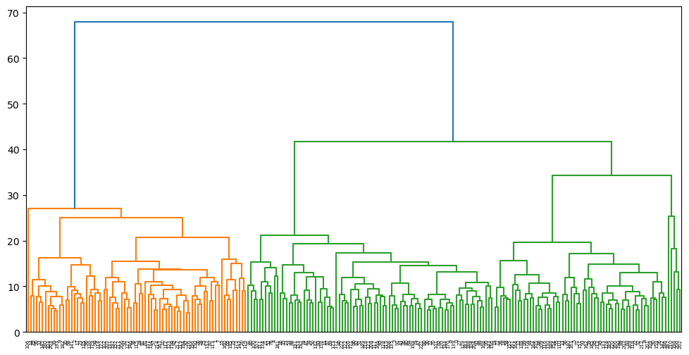
We have also observed that the input features are correlated. Hence when we applied PCA the correlation got removed. We chose the first 11 PCAs to be a useful one. Then we fitted KMeans and chose 2 clusters by knee bend plot. We have also used hierarchical clustering and went with 2 clusters.
Models
We have fitted 7 models from linear additive to interaction. Calculated its coefficients and showed statistical significance. We decided on the good models over the number of coefficients, threshold, Accuracy, Sensitivity, Specificity, FPR, and ROC_AUC. This was based on a test dataset.
    formula_linear = 'Y ~ ' + ' + '.join(df_standardized_transformed.drop(columns= 'Y').columns)
    mod_03 = smf.ols(formula=formula_linear, data=df_standardized_transformed).fit()
    mod_03.params
    # Apply PCA to the transformed inputs and create all pairwise interactions between the PCs.
    df_pca_transformed_int = df_pca_transformed.iloc[:, :11].copy()
    df_pca_transformed_int['Y'] = df_transformed.Y
    formula_int = 'Y ~ ' + ' ( '  + ' + '.join(df_pca_transformed_int.drop(columns= 'Y').columns) + ' ) ** 2'
    mod_07 = smf.ols(formula=formula_int, data=df_pca_transformed_int).fit()
    mod_07.params
We chose model 3 and model 7 from there which are all linear additive features from the original data set and model 7 is the interaction features with PCAs. They have 64 and 67 coefficients respectively.
Prediction
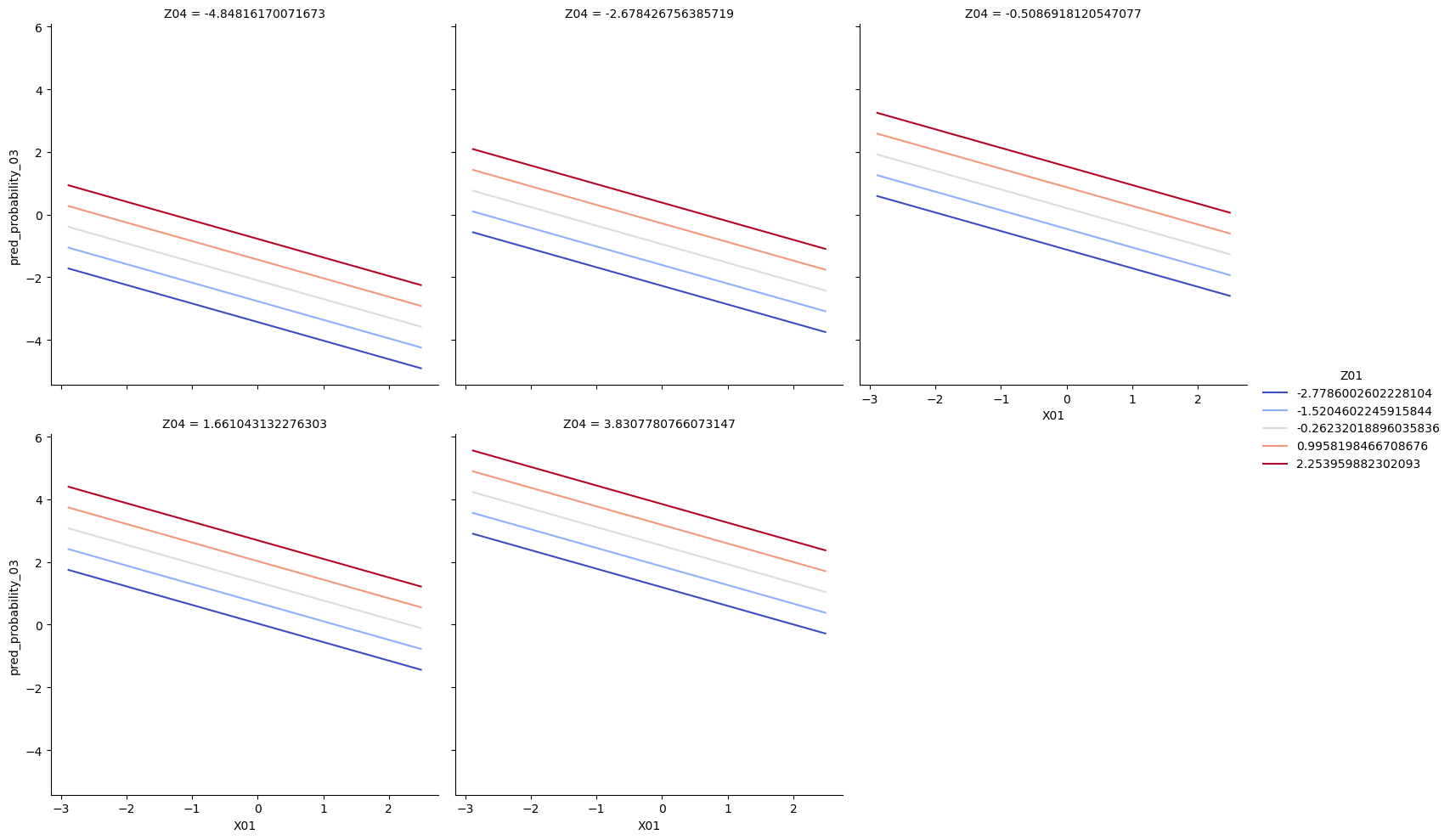
Recall we had only training data with us. Hence, we chose model 3 and model 7 to check them on the test dataset that was created by us manually in the input grids X01, Z01, and Z04. Then we had prediction in model 3 we drew some line prediction plots for model 3 with x=’X01’, y=’pred_probability_03’, hue=’Z01’, and col=’Z04’.
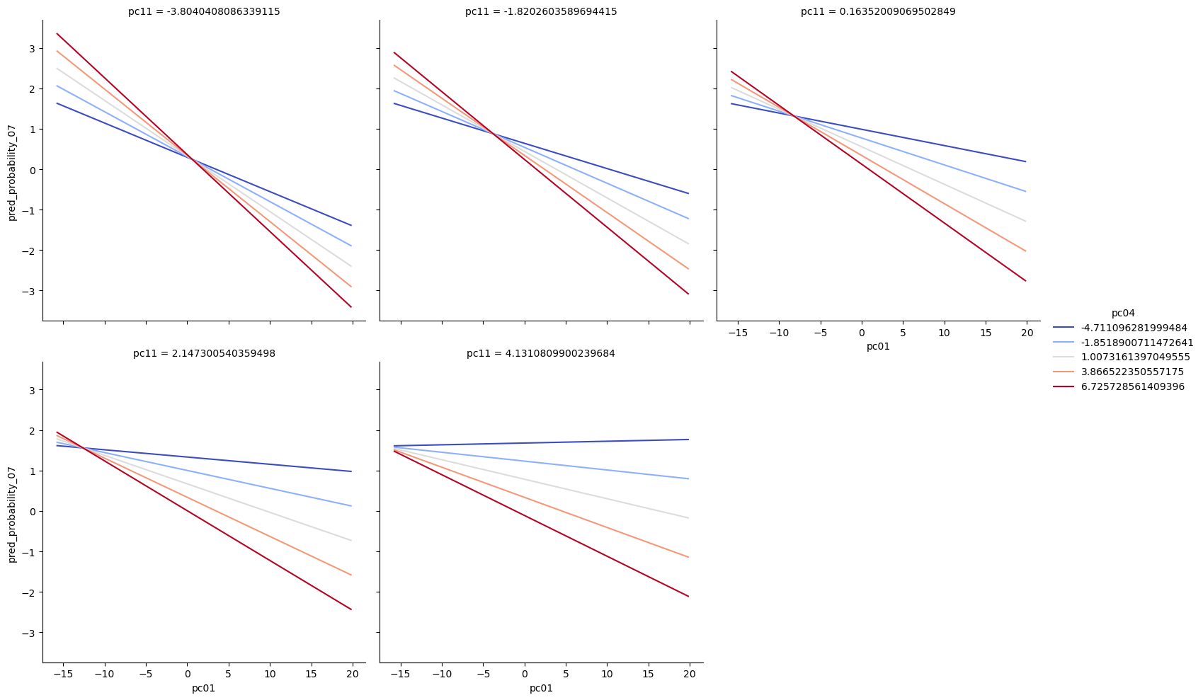
Next, we had prediction in model 7 we drew some line prediction plots for model 7 with x=’pc01’, y=’pred_probability_07’, hue=’pc04’, col=’pc11’.
Performance
Next, we evaluated performance with Pipelines fitting logistic regression along with regularization lasso, ridge, and elastic net. We did not restrict ourselves strictly to lasso or ridge, rather went for an elastic net. From the l1 ratio, we observed that it is leaning towards lasso. Hence, we calculated performance with lasso and we got the highest score as 84%.
  # model 7-Apply PCA to the transformed inputs and create all pairwise interactions between the PCs
  pc_interact_lasso_search_grid.best_score_

0.8387878787878786
At the end, we forced to do elestic net a grid search with l1 ratio 0.5. Here also we got 84% accurate with 31 features coefficient zero. Hence we call it the best.
  enet_to_fit = LogisticRegression(penalty='elasticnet', solver='saga',
                            random_state=202, max_iter=25001, fit_intercept=True)
  pc_interact_enet_wflow = Pipeline( steps=[('std_inputs', StandardScaler() ),
                                           ('pca', PCA() ),
                                           ('make_pairs', make_pairs),
                                           ('enet', enet_to_fit )] )
  enet_grid = {'pca__n_components': [3, 5, 7, 9, 11, 13, 15, 17],
             'enet__C': np.exp( np.linspace(-10, 10, num=17)),
             'enet__l1_ratio': np.linspace(0, 1, num=3)}
  pc_df_enet_search = GridSearchCV(pc_interact_enet_wflow, param_grid=enet_grid, cv=kf)
  pc_df__enet_search_results = pc_df_enet_search.fit( x_train_transformed, y_train_transformed )
  #The optimal value for C and no. of pca components is
  pc_df__enet_search_results.best_params_
  pc_df__enet_search_results.best_score_
0.8387878787878786
0.8387878787878786
  coef = pc_df__enet_search_results.best_estimator_.named_steps['enet'].coef_
  empty_elements = coef[coef == 0]
  empty_elements.size
31
Extra
We have also fitted SVC and Neural net. In neural net we got 91% to 100% accuracy over cross validation and in SVC we get 100% accuracy all the time.
SVC
  svm_model = SVC()

  svm_param_grid = {
      'C': [0.1, 1, 10, 100],
      'kernel': ['linear', 'rbf', 'poly'],
      'gamma': ['scale', 'auto']
  }

  svm_result=svm_grid_search.fit(x_train_transformed, y_train_transformed)
  svm_result.best_params_

  svm_result.best_score_
  svm_cross_val_scores = cross_val_score(svm_grid_search.best_estimator_, x_train_transformed, y_train_transformed, cv=5, scoring='accuracy')
  print("SVM Cross-Validation Scores:", svm_cross_val_scores)
  print("SVM Mean Cross-Validation Score:", svm_cross_val_scores.mean())
SVM Cross-Validation Scores: [1. 1. 1. 1. 1.]
SVM Mean Cross-Validation Score: 1.0
Neural Net
  # Appropriate model based on our task (regression/classification) is
  # RandomForestClassifier for classification(RandomForestRegressor for regression )
  model = RandomForestClassifier()

  # Define the parameter grid for tuning
  param_grid = {
    'n_estimators': [50, 100, 200],
    'max_depth': [None, 10, 20, 30],
    'min_samples_split': [2, 5, 10],
    'min_samples_leaf': [1, 2, 4]
  }

  # Create the GridSearchCV object
  grid_search = GridSearchCV(model, param_grid, cv=5, scoring='accuracy')  # Use appropriate scoring for your task

  # Fit the grid search to your data
  grid_search.fit(x_train_transformed, y_train_transformed)

  # Get the best parameters
  best_params = grid_search.best_params_
  print("Best Parameters:", best_params)

  # Assess performance using cross-validation
  cross_val_scores = cross_val_score(grid_search.best_estimator_, x_train_transformed, y_train_transformed, cv=5, scoring='accuracy')  # Use
  appropriate scoring
  print("Cross-Validation Scores:", cross_val_scores)
  print("Mean Cross-Validation Score:", cross_val_scores.mean())
Cross-Validation Scores: [1.         1.         0.95555556 0.90909091 1.        ]
Mean Cross-Validation Score: 0.972929292929293
Summary
In EDA we saw the inputs are highly correlated and that’s why they are not very good at separating Y=0,1. The KMeans k2=0,1 worked well and it was not only giving us a better hue in the scatter plot but also matched well with Y=0,1.
We can see that V07, V15, X10 are statistically significant features. It seems the 3rd approach to extracting patterns from the signals is more useful.
Because they are correlated to each other we need the help of PCA to evaluate effective feature variables and at the end, we saw that there are 11 to 13 such PCA features that separate the data well and, hence, effective.
The best logistic regression model turns out to be the elastic net with even mixed with ridge and lasso with 31 zero coefficients. We are getting 83-84% accuracy here. The best model in training turns out to be the best in prediction as well. In the end we saw if we use SVC then we are in fact getting 100% accuracy. I have also included Neural Net in the supporting document where we get 97% accuracy.
Things to answer and to be updated next
This was my second project and more things are yet to be learned and improved. Data Science/machine learning is a journey like life
- Removing skew with data-independent approach
- How to choose optimal no PCA
- More advanced methods after logistic regression.
References
- University of Pittsburgh course CMPINF 2100
- VSCode, Python
💻